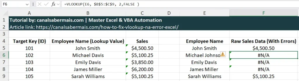
Did you carefully set up your VLOOKUP formula only to be blocked by the frustrating #N/A error? You are not alone. In fast-paced corporate environments, it is incredibly common to overlook small structural adjustments that make all the difference in your final calculation outputs.
Fortunately, you can eliminate this disruption instantly. Discover 4 simple methods to identify, troubleshoot, and bypass these common spreadsheet mismatches, making your reporting models significantly more robust and professional.
Download the Free Practice Spreadsheet
📥 Want to follow along with this tutorial? Click here to download the exact Excel spreadsheet used in this guide. Open the file now to practice and fix your formulas in real-time as you read.
The Quick Fix: Using IFERROR with VLOOKUP
The fastest and most efficient way to handle missing data and keep your worksheets clean is by nesting your formula inside the IFERROR function. This method acts as a technical safety net, replacing the ugly error code with a clean, professional text message or a neutral zero value.
Instead of using a standard formula, apply the following structured layout to maintain data integrity:
=IFERROR(VLOOKUP(E5, B5:C9, 2, FALSE), "Not found")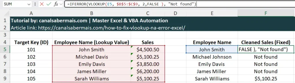
By using this approach, if the lookup values do not match, Excel will display “Not Found” instead of throwing a system error, allowing your remaining column operations and financial forecasts to calculate seamlessly.
Common Causes and Technical Solutions
If you need to identify exactly why your database is failing to match entries, you must audit the data structure. Below are the three most common hidden discrepancies found in corporate environments and how to fix them.
1. Trailing Spaces and Hidden Characters
One of the main reasons a VLOOKUP fails is the presence of invisible trailing spaces or non-printing characters within the data cell. To the human eye, “John Smith” and “John Smith ” look identical, but to the Excel lookup engine, they are entirely different arrays.
To eliminate these invisible roadblocks instantly, combine VLOOKUP with the TRIM function as shown below:
=VLOOKUP(TRIM(E7), B5:C9, 2, FALSE)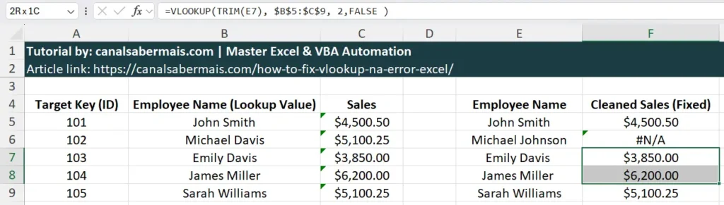
The TRIM function dynamically strips away any accidental leading or trailing spaces from the target cell before running the lookup query, ensuring an exact matching process.
2. Mismatched Data Types (Text vs. Numbers)
Another classic spreadsheet mismatch happens when your lookup value is formatted as a true number, but the corresponding value in the source database array is stored as text (or vice versa). Excel cannot map cross-type records automatically.
Review the standard structural mismatch in the comparative matrix below:
| Lookup Value Status | Source Database Status | System Result |
|---|---|---|
| 102 (True Number) | “102” (Text Format) | #N/A Error |
| 102 (True Number) | 102 (True Number) | Successful Match |
=VLOOKUP(E6, A5:C9, 3, FALSE)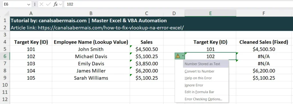
To resolve this database formatting issue without changing the original source properties, use the VALUE function to force textual digits into numerical formats during execution:
=VLOOKUP(VALUE(E6), A5:C9, 3, FALSE)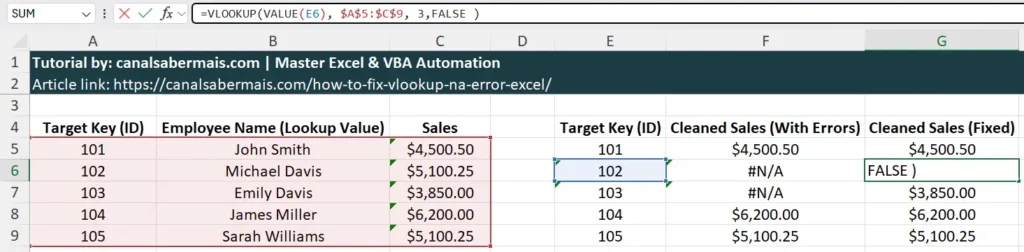
3. Approximate Match vs. Exact Match
If the final argument of your VLOOKUP formula is omitted or set to TRUE, Excel defaults to an approximate match behavior. This means the system requires your first reference column to be sorted in strict ascending order to function correctly. If it is unsorted, the formula yields a false #N/A indication.
=IFERROR(VLOOKUP(E5, B5:C9, 2, TRUE), "Not found")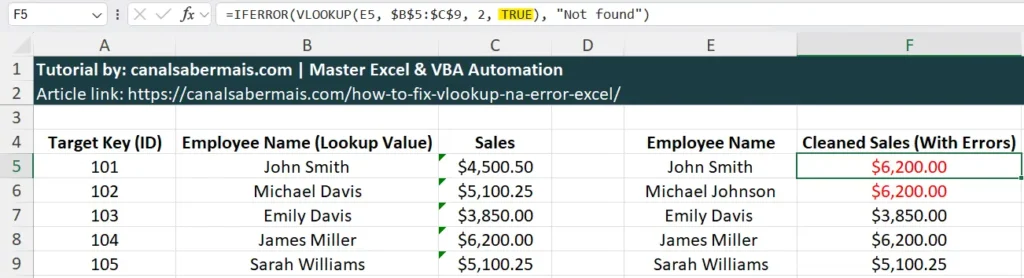
To avoid this database mapping pitfall, always explicitly declare a strict exact match routine by forcing the fourth argument to FALSE or 0:
=IFERROR(VLOOKUP(E5, B5:C9, 2, FALSE), "Not found")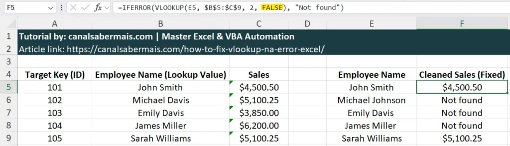
Frequently Asked Questions (FAQ)
Why does VLOOKUP return #N/A when the lookup value is clearly visible in the worksheet?
This structural mismatch typically happens due to hidden trailing spaces or a data type discrepancy. If your target lookup identifier is formatted as text but the source data array holds a true numerical value, the search engine fails to execute a match and throws the error code.
Is there a performance difference between using IFERROR and migrating to XLOOKUP?
Yes. Nesting VLOOKUP inside an IFERROR block forces the system to run two calculations sequentially. Upgrading to XLOOKUP allows you to handle missing spreadsheet elements natively using its internal [if_not_found] parameter, optimizing processing speeds on large databases.
How do I force VLOOKUP to run a strict exact match procedure by default?
To secure a rigid match routine across unsorted reference data arrays, you must explicitly declare the fourth argument (range_lookup) of your formula as FALSE or 0. Omitting this statement causes Excel to execute a flawed approximate match check.
Can the TRIM function remove non-breaking web spaces from imported databases?
No. The standard TRIM function only clears standard ASCII white spaces (character code 32). For databases extracted from enterprise web platforms or ERP systems containing non-breaking spaces (character code 160), you must combine the SUBSTITUTE function with your lookup routine.
Worksheet Autonomy and Data Integrity
As we have explored, auditing your source database is a critical step in sheet optimization. Furthermore, implementing minor precautions when developing your formulas can significantly help you build more robust and reliable corporate dashboards.
Proactively handling recurring formatting glitches—such as stripping extra whitespaces and displaying a clean fallback message like “Not Found”—not only shields your worksheets from unexpected calculation breakdowns but also ensures your business reports command maximum credibility.