Performing complex data lookups using multiple columns as search criteria can quickly get complicated. Traditionally, you would either create a helper column to concatenate data or rely on clunky, less effective workarounds. In this quick guide, you will learn how to use XLOOKUP with multiple criteria to streamline your workflow and upgrade your spreadsheet efficiency.
Download the Free Practice Spreadsheet
📥 Want to follow along with this tutorial? Click here to download the exact Excel spreadsheet used in this guide. Open the file now to practice and fix your formulas in real-time as you read.
The Core Syntax for XLOOKUP with Multiple Criteria
To master how to use XLOOKUP with multiple criteria without using helper columns, you must use Excel’s boolean logic inside the function. Instead of searching for a single value, an advanced XLOOKUP multiple criteria formula evaluates multiple arrays and multiplies the conditions using the (array1=criteria1)*(array2=criteria2) structure.
When Excel evaluates these arrays, true matches convert to 1 and mismatches convert to 0. By multiplying them, a row where all criteria are true yields a 1, which the function intercepts instantly.
=XLOOKUP(1, (Array1=Criteria1) * (Array2=Criteria2), ReturnArray, "Not Found", 0)(A5:A13=G4) -> {FALSE;FALSE;FALSE;TRUE;TRUE;TRUE;FALSE;FALSE;FALSE}
(B5:B13=G5) -> {TRUE;FALSE;FALSE;TRUE;FALSE;FALSE;TRUE;FALSE;FALSE}
Result -> {0;0;0;1;0;0;0;0;0}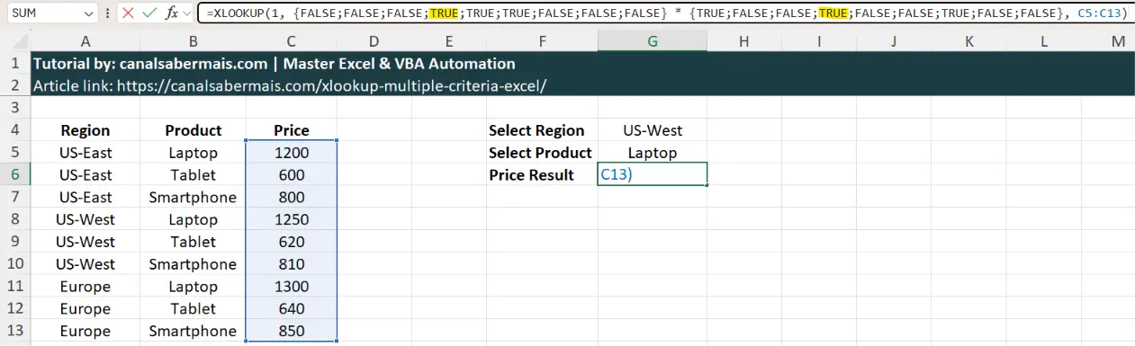
Step-by-Step Practical Application
Imagine you run a corporate inventory database where items are categorized by both a “Region” and a “Product”. You need to find the exact price for a specific item matching both criteria simultaneously.
| Region (Col A) | Product (Col B) | Price (Col C) |
|---|---|---|
| US-East | Laptop | $1,200.00 |
| US-West | Laptop | $1,250.00 |
| Europe | Tablet | $640.00 |
To extract the unit price for a “Laptop” in the “US-West” region located in cell G4 and G5 respectively, apply the formula block using exact array multiplication definitions:
=XLOOKUP(1, (A5:A13=G4) * (B5:B13=G5), C5:C13)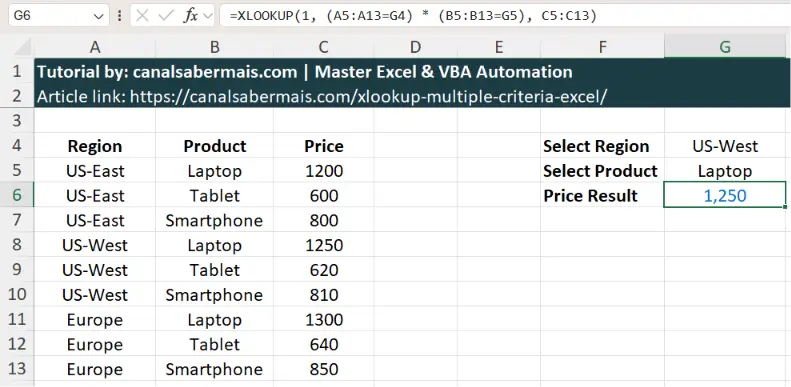
Why VLOOKUP Fails with Multiple Conditions
Traditional lookup functions like VLOOKUP are structurally limited to searching a single column. For years, financial analysts were forced to combine text values using ampersands (e.g., =A2&B2) to build synthetic lookup targets.
This dynamic workaround is highly inefficient for large datasets, as it forces Excel to recalculate thousands of unnecessary data strings, lagging your corporate files and operational systems.
- No Helper Columns: Keeps your raw source tables completely clean.
- Exact Matching: Evaluates data points natively without character blending errors.
- Performance Boost: Processes boolean arrays faster inside memory storage.
Troubleshooting Common XLOOKUP Logic Errors
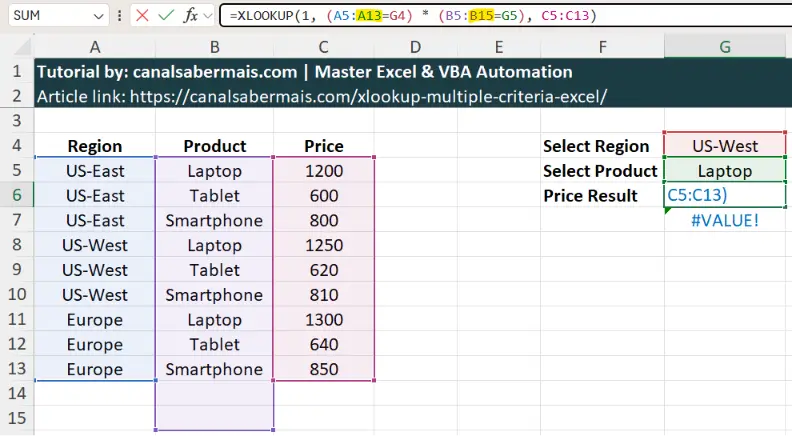
If your multiple criteria formula returns an unexpected #VALUE! error, the problem is almost always an asymmetrical array sizing structure. Excel requires all conditional evaluation ranges inside the lookup argument to have identical horizontal or vertical lengths.
For example, if your first evaluation criteria spans range A5:A13 but your second criteria accidentally targets B5:B15, the system cannot perform row-by-row boolean math, causing the calculation to break instantly.
Additionally, always ensure you isolate each separate match condition within its own set of parentheses before applying the asterisk (*) operator to properly preserve mathematical hierarchies.
Frequently Asked Questions (FAQ)
1. Why do we look for the number 1 in a multiple criteria XLOOKUP?
When you implement an advanced XLOOKUP multiple criteria formula, Excel evaluates each condition inside parentheses and returns arrays of TRUE or FALSE values. In programming logic, TRUE equals 1 and FALSE equals 0. By multiplying these arrays with an asterisk (*), a row where all conditions are met yields 1 * 1 = 1. Searching for 1 allows the function to pinpoint that exact logical match instantly.
2. Can I use this boolean logic method with more than two criteria?
Yes. You can add as many conditions as your corporate database requires. Simply follow the exact same syntax pattern by multiplying another conditional array:
=XLOOKUP(1, (Array1=Criteria1) * (Array2=Criteria2) * (Array3=Criteria3), ReturnArray)Just make sure all evaluation ranges span identical row lengths.
3. Does using multiple criteria inside XLOOKUP slow down large spreadsheets?
No, it is highly optimized. Because it processes boolean arrays natively in memory, it is significantly faster and lighter than legacy alternatives like creating physical helper columns or utilizing nested array formulas, protecting your system performance.
4. Why does my multiple criteria formula return a #VALUE! error?
This error almost always happens when your lookup arrays are asymmetrical. If your first lookup range is A5:A13 but your second range is accidentally typed as B5:B15, Excel cannot perform row-by-row binary multiplication and the formula breaks instantly.
Conclusion: Driving Efficiency with Boolean Lookup Logic
Mastering boolean logic is a natural step for professionals building advanced formulas to extract the full potential of their data. Applying the (1)*(1) logic to XLOOKUP provides a clean, robust solution that eliminates helper columns. This method saves valuable office time while delivering powerful, easy-to-read formulas for corporate data analysis.